Mastering Logistic Regression for Predictive Analysis
Unlock the Power of Binary Classification

1. Understanding Logistic Regression
Logistic regression is a powerful statistical model commonly used to analyze binary outcomes. In essence, logistic regression employs a logistic function to estimate the probability of an event occurring or not. Although this method primarily deals with binary dependent variables, it can be extended to handle more complex scenarios as well.
A binary logistic model focuses on a dependent variable that has two possible outcomes, such as pass/fail or success/failure. These outcomes are represented using indicator variables ‘0’ and ‘1’. The logistic model predicts the log-odds (the logarithm of the odds) of the outcome labeled ‘1’, which depends on one or more independent variables, also known as predictors. These predictors can either be binary variables or continuous variables.
The conversion of log-odds to probabilities is carried out by the logistic function, hence the name “logistic regression”. The unit of measurement for the log-odds scale is known as a logit or logistic unit, which contributes to the alternative names for this method.
In a logistic model, increasing one of the independent variables will multiplicatively scale the odds of the given outcome at a constant rate. Each independent variable has its own parameter, and when dealing with binary independent variables, this generalizes the concept of odds ratio.
It’s important to note that variations of logistic regression exist, such as the probit model, which uses a different sigmoid function instead of the logistic function. However, the defining characteristic of logistic regression is its ability to model the relationship between independent variables and the probability of a binary outcome.
1.1 The Importance of Log-Odds in Logistic Regression
Before exploring betting odds, it’s crucial to grasp the concept of log-odds and their significance in logistic regression. Log-odds are a transformation of probabilities that enables them to range from very small negative values to very large positive values. This transformation allows logistic regression models to predict the log-odds using input features. These predictions are then employed to classify examples into different categories.
The log-odds of an event can be calculated by taking the logarithm of the odds ratio. The odds ratio is defined as the probability of an event occurring divided by the probability of it not occurring. This is also known as the logit function. Mathematically, this can be represented as:
$$ \mathrm{log_odds} = \log\left(\frac{p}{1-p}\right) $$
where $p$ is the probability of an event occurring.
In Python, we can define a logit() function that calculates the log-odds values given a set of probabilities.
import numpy as np

def logit(probs):
    odds = probs / (1 - probs)
    log_odds = np.log(odds)
    return log_odds
This logit() function will take an array of probabilities and return an array of log-odds values. By providing a better understanding of the relationship between probabilities and log-odds, this function serves as a useful tool for interpreting betting odds within the context of logistic regression.
1.2 Betting Odds and Expected Value of Winnings
Gambling involves betting on uncertain outcomes, making it essential to understand the expected value of winnings when determining a fair wager. The expected value of winnings takes into account the probabilities of different outcomes and their associated monetary values to calculate the average amount one can expect to win in the long run.
Consider a simple card game involving a deck containing nine spades and one heart. The aim is to draw a card; if the heart is drawn, the player wins, otherwise, the dealer wins. This setup results in a 10% probability or 1:9 odds of the player winning.
A fair wager is one where both parties expect to win the same amount in the long run. We can calculate this using the expected value of winnings formula:
$$Expected~Value~of~Winnings = \boldsymbol{p} \cdot \boldsymbol{v}$$
where $\boldsymbol{p}$ is a vector of probabilities for each outcome, and $\boldsymbol{v}$ is a vector of dollar-values for each outcome.
In this example, there are two possible outcomes: win or lose. Therefore, $\boldsymbol{p}$ would be a 2-dimensional vector with the probabilities of winning and losing, and $\boldsymbol{v}$ would also be a 2-dimensional vector with the dollar-values for winning and losing. We can represent these vectors as:
$$\boldsymbol{p} = \begin{bmatrix}
0.1 \
0.9
\end{bmatrix},~~\boldsymbol{v} = \begin{bmatrix}
10 \
-10
\end{bmatrix}$$
The player has a 10% chance of winning and a 90% chance of losing, with a possible win of $10 and a loss of $10. Using the formula for expected value of winnings, we can calculate the average amount someone can expect to win in the long run:
$$Expected~Value~of~Winnings = (0.1 \times 10) + (0.9 \times -10) = -8$$
On average, a player can expect to lose $8 if they repeatedly play this game.
If both parties agree to wager $10, we can use the same formula to calculate their expected winnings. However, since the odds of winning favor the dealer, they should stake less money than the player to balance things out. For instance, if the dealer bets $5 and the player bets $10, we can calculate their expected winnings as follows:
#Player/Dealer Winnings
import numpy as np

p = np.array([0.1, 0.9])           # array of probabilities [p_w, p_l]
v = np.array([10, -10])            # array of dollar-values [v_w, v_l]
wager = np.array([5, 10])          # array of wagers [dealer, player]

expected_winnings = np.dot(p * v, wager)

DealerWinnings = (0.9 * +5) + (0.1 * -5)
PlayerWinnings = (0.1 * +10) + (0.9 * -10)
print(DealerWinnings)
print(PlayerWinnings)
4.0
-8.0
Example Scenario: In this betting scenario, the dealer is expected to win $4, while the player is expected to lose $8. By staking less money, the dealer reduces their potential winnings but also minimizes their potential losses due to the unfavorable odds. This example highlights the significance of understanding probabilities and the expected value of winnings when deciding on a fair wager. Building on this idea, it becomes crucial to analyze different betting scenarios and visualize their potential outcomes to make informed decisions. The following guide explains how to create a DataFrame for such visualizations.
1.2.1 Significance of the DataFrame and Visualization
The following Python code generates a DataFrame that calculates and visualizes the expected winnings for various betting scenarios between a player and a dealer. This DataFrame (df) is useful for understanding the impact of different betting combinations on the potential outcome for the player. It simplifies the decision-making process by highlighting the best betting scenario, where the player can maximize their expected winnings.
1.2.1.1 Key Components of DataFrame Visualization
-
Dimensions: The resulting DataFrame has dimensions
(len(base_bets), len(base_bets)), wherebase_betsis an array of odd integers from 1 to 11. Each row in the DataFrame corresponds to a possible bet placed by the dealer, while each column corresponds to a possible bet placed by the player. -
Expected Winnings Calculation: For each betting scenario, the expected winnings are calculated using a fixed probability model, assuming a 10% chance of the player winning 90% of the dealer’s bet and a 90% chance of the player losing their bet. These calculations are stored in a 2D NumPy array called
player_winnings. -
Betting Scenarios Representation: The Python code uses pandas to create a DataFrame that displays the expected winnings for each scenario in a tabular format. The DataFrame has rows labeled as “Dealer Bet” and columns labeled as “Player Bet”. This elegant representation makes it easy to identify the optimal betting combination, maximizing the chances of winning for the player.
Using this information, anyone interested in analyzing different betting situations can easily view the potential outcomes and make informed decisions based on the presented data. The DataFrame acts as a tool to visualize and better comprehend these complex relationships between probabilities and expected winnings.
# Expected Winnings DF
import numpy as np
import pandas as pd

def simple_argmax(arr):
    '''helper to convert np.argmax into something usable'''
    return np.array(np.unravel_index(np.argmax(arr), arr.shape))

def df_names(df, idxs):
    '''helper to convert number of index/column labels'''
    r,c = idxs
    return df.index[r], df.columns[c]

base_bets = np.arange(1,12,2)
player_bet, dealer_bet = np.meshgrid(base_bets, base_bets)
player_winnings = .1 * dealer_bet + .9 * -player_bet
df = pd.DataFrame(player_winnings, index=base_bets, columns=base_bets)
df.index.name = "Dealer Bet"
df.columns.name = "Player Bet"
print("Best Betting Scenario (for Player) for These Values:")
print("(Dealer, Player):", df_names(df, simple_argmax(player_winnings)))
df
Best Betting Scenario (for Player) for These Values:
(Dealer, Player): (11, 1)
| Player Bet | 1 | 3 | 5 | 7 | 9 | 11 |
|---|---|---|---|---|---|---|
| Dealer Bet | ||||||
| 1 | -0.8 | -2.6 | -4.4 | -6.2 | -8.0 | -9.8 |
| 3 | -0.6 | -2.4 | -4.2 | -6.0 | -7.8 | -9.6 |
| 5 | -0.4 | -2.2 | -4.0 | -5.8 | -7.6 | -9.4 |
| 7 | -0.2 | -2.0 | -3.8 | -5.6 | -7.4 | -9.2 |
| 9 | 0.0 | -1.8 | -3.6 | -5.4 | -7.2 | -9.0 |
| 11 | 0.2 | -1.6 | -3.4 | -5.2 | -7.0 | -8.8 |
1.2.2 Moneyline Betting and Its Relation to the Simple Game
In the simple game, the odds are 1:9, meaning the probability of winning is 1 out of 10 (or 10%), and the probability of losing is 9 out of 10 (or 90%). In Moneyline betting, these probabilities are represented differently. Instead of saying “the probability of winning is 10%”, the odds are represented in terms of how much money you would win or need to wager.
Let’s use the example of George St. Pierre (-190) vs. Michael Bisping (+175):
- The negative number (-190) for George St. Pierre means he is the favorite, and you would need to bet $190 to win $100. This implies that the probability of him winning is high.
- The positive number (+175) for Michael Bisping means he is the underdog, and you would win $175 if you bet $100. This implies that the probability of him winning is lower.
To relate this to the simple game, let’s say the dealer is like George St. Pierre and the player is like Michael Bisping.
- If you bet $10 on the dealer (like betting on George St. Pierre), you would win $1 (10% of $10) if the dealer wins (like if George St. Pierre wins), but lose $9 (90% of $10) if the dealer loses (like if George St. Pierre loses).
- If you bet $10 on the player (like betting on Michael Bisping), you would win $9 (90% of $10) if the player wins (like if Michael Bisping wins), but lose $1 (10% of $10) if the player loses (like if Michael Bisping loses).
So, in both the simple game and Moneyline betting, the amount you win or lose is proportional to the odds (or probabilities) of winning or losing. The main difference is in how the odds are represented.
In the case of the 1:9 odds from the simple game, the situation is heavily skewed towards the dealer (the “favorite”), with the player being the “underdog”. To convert these odds to Moneyline format, we need to determine the implied probabilities and then convert those probabilities to Moneyline odds.
The implied probability for the favorite (dealer) winning is 9/10 = 0.9 or 90%. The implied probability for the underdog (player) winning is 1/10 = 0.1 or 10%.
The formula to convert these probabilities to Moneyline odds is:
- For the favorite (probability > 50%): Moneyline Odds = - (100 / (Implied Probability) - 100)
- For the underdog (probability < 50%): Moneyline Odds = 100 / (1 - Implied Probability) - 100
Using these formulas, the Moneyline odds would be:
- For the favorite (dealer): -900 (you would need to bet $900 to win $100)
- For the underdog (player): +900 (you would win $900 if you bet $100)
Please note that these are simplified calculations and actual Moneyline odds may vary based on various factors including the sportsbook’s margin.
1.2.3 Converting Moneyline Odds to Ratios
It is possible to convert Moneyline odds to probability, which can then be represented as ratios similar to the simple game. Here’s how you can do it:
-
Convert Moneyline odds to probability:
For a favorite (negative Moneyline odds), the formula is: Probability = - (Moneyline Odds) / ((- (Moneyline Odds)) + 100)
For an underdog (positive Moneyline odds), the formula is: Probability = 100 / (Moneyline Odds + 100)
Using these formulas, the probabilities for George St. Pierre (-190) and Michael Bisping (+175) would be:
- George St. Pierre: - (-190) / ((- (-190)) + 100) = 0.655 or 65.5%
- Michael Bisping: 100 / (175 + 100) = 0.364 or 36.4%
Please note that these probabilities do not add up to 100% due to the bookmaker’s overround (also known as the vig or juice), which is the way bookmakers make a profit.
-
Convert probabilities to ratios:
The ratios can be found by dividing the probability of each outcome by the probability of the other outcome.
- Ratio for George St. Pierre: Probability of George St. Pierre / Probability of Michael Bisping = 0.655 / 0.364 = 1.8
- Ratio for Michael Bisping: Probability of Michael Bisping / Probability of George St. Pierre = 0.364 / 0.655 = 0.56
These ratios are similar to the 1:9 odds in the simple game, but they represent a much closer contest.
Please note that these calculations are simplified and actual odds and probabilities may vary based on various factors including the sportsbook’s margin.
1.3 Understanding Probabilities, Odds, and Log-Odds: The Foundation of Logistic Regression
When it comes to betting scenarios, odds are a common term that helps us understand the likelihood of an event occurring. The odds of an event are calculated as the ratio of the probability of the event happening (p) to the probability of the event not happening (1 - p). For example, if the probability of winning a game is 10% (p = 0.1), the odds of winning would be 1:9. This means that for every one time we expect to win, we expect to lose nine times.
1.3.1 Introducing Log-Odds
Log-odds is the natural logarithm of the odds. It plays a crucial role in logistic regression as it serves as a format for representing probabilities suitable for linear regression methods. Providing a continuous function ranging from negative infinity to positive infinity, log-odds fit nicely with the linear equation used in linear regression models.
To further illustrate this concept, let’s look at a few sample probability values, their respective odds, and log-odds:
| Probability | Odds | Log-Odds |
|---|---|---|
| 0.1 | 1:9 | -2.1972 |
| 0.5 | 1:1 | 0 |
| 0.9 | 9:1 | 2.1972 |
The code below defines a set of probability values, calculates their corresponding odds and log-odds, and presents the results in a pandas DataFrame.
-
Defining probabilities: First, the code defines various probabilities (
tail_probs,lwr_probs,upr_probs, andcent_prob). Then, it concatenates these probabilities to create a single array of probabilities,probs. -
Calculating odds and log-odds: With np.errstate(), the code suppresses warnings that may arise due to division by zero. It computes the odds by dividing each probability by its complementary probability, i.e.,
odds = probs / (1 - probs). The log-odds are then calculated using numpy’s log function:log_odds = np.log(odds). -
Creating a DataFrame: The code creates a list of index labels by formatting the probabilities as percentages. It then constructs an OrderedDict to create the DataFrame columns and their corresponding data. Finally, it creates a pandas DataFrame using the
polo_dictand the index labels. The DataFrame displays the probability (Prob(E)), odds (Odds(E:not E)), and log-odds (Log-Odds) for each percentage value (Pct(%)).
The output DataFrame shows the relationship between the probability values, odds, and log-odds. Keep in mind that the log-odds are calculated as the natural logarithm of the odds (using numpy’s np.log function).
from collections import OrderedDict

tail_probs = [0.0, .001, .01, .05, .10, .25, 1.0/3.0]
lwr_probs = np.array(tail_probs)
upr_probs = 1-lwr_probs[::-1]
cent_prob = np.array([.5])
probs = np.concatenate([lwr_probs, cent_prob, upr_probs])

# Compute odds and log-odds
with np.errstate(divide='ignore'):
    odds = probs / (1-probs)
    log_odds = np.log(odds)

index=["{:4.1f}%".format(p) for p in np.round(probs,3)*100]
polo_dict = OrderedDict([("Prob(E)", probs), ("Odds(E:not E)", odds), ("Log-Odds", log_odds)])
polo_df = pd.DataFrame(polo_dict, index=index)
polo_df.index.name="Pct(%)"
polo_df
| Prob(E) | Odds(E:not E) | Log-Odds | |
|---|---|---|---|
| Pct(%) | |||
| 0.0% | 0.000000 | 0.000000 | -inf |
| 0.1% | 0.001000 | 0.001001 | -6.906755 |
| 1.0% | 0.010000 | 0.010101 | -4.595120 |
| 5.0% | 0.050000 | 0.052632 | -2.944439 |
| 10.0% | 0.100000 | 0.111111 | -2.197225 |
| 25.0% | 0.250000 | 0.333333 | -1.098612 |
| 33.3% | 0.333333 | 0.500000 | -0.693147 |
| 50.0% | 0.500000 | 1.000000 | 0.000000 |
| 66.7% | 0.666667 | 2.000000 | 0.693147 |
| 75.0% | 0.750000 | 3.000000 | 1.098612 |
| 90.0% | 0.900000 | 9.000000 | 2.197225 |
| 95.0% | 0.950000 | 19.000000 | 2.944439 |
| 99.0% | 0.990000 | 99.000000 | 4.595120 |
| 99.9% | 0.999000 | 999.000000 | 6.906755 |
| 100.0% | 1.000000 | inf | inf |
The code below creates a DataFrame displaying the minimum and maximum values of the columns in polo_df. This provides an overview of the range of values in each column.
pd.DataFrame([polo_df.min(axis=0), polo_df.max(axis=0)], index=['min', 'max']).T
| min | max | |
|---|---|---|
| Prob(E) | 0.0 | 1.0 |
| Odds(E:not E) | 0.0 | inf |
| Log-Odds | -inf | inf |
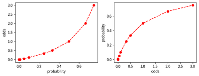
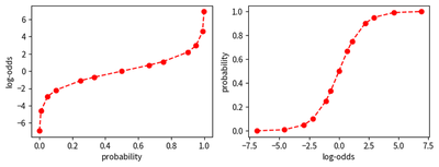
The relationships among probability, odds, and log-odds can be visualized through graphs, which demonstrate a mutual increase. However, while the relationship between probability and log-odds is linear, the same cannot be said for probability and odds. The linear nature of log-odds makes it a perfect candidate for use in logistic regression. The following code plots four graphs to illustrate the relationships between probability, odds, and log-odds:
-
Define a helper function: A helper function
helper()is defined to plot the graphs easily. The function takes input parametersax(axis),x,y,x_name, andy_name. It plots a red dashed line with circles, labels the x-axis and y-axis with provided names, and set the axes properties accordingly. -
Create subplots: Using
plt.subplots(), the code creates two sets of subplots side by side on separate figures, with each set containing two graphs. Thefigsizeparameter sets the size of the figures. -
Plot graphs: The code uses the helper function to plot four graphs:
- Probability vs. Odds: The first graph plots the probability on the x-axis and the odds on the y-axis. It helps in visualizing how the odds change with respect to probability.
- Odds vs. Probability: The second graph is the inverse of the first one, plotting the odds on the x-axis and the probability on the y-axis.
- Probability vs. Log-Odds: The third graph plots the probability on the x-axis and log-odds on the y-axis. It showcases the relationship between probabilities and their corresponding log-odds values.
- Log-Odds vs. Probability: The fourth graph is the inverse of the third one, plotting the log-odds on the x-axis and the probability on the y-axis.
import matplotlib.pyplot as plt
import collections as co

def helper(ax, x, y, x_name, y_name):
    ax.plot(x, y, 'r--o')
    ax.set_xlabel(x_name)
    ax.set_ylabel(y_name)

fig, (ax0, ax1) = plt.subplots(1, 2, figsize=(9, 3))
helper(ax0, probs[:-5], odds[:-5], 'probability', 'odds')
helper(ax1, odds[:-5], probs[:-5], 'odds', 'probability')

fig, (ax0, ax1) = plt.subplots(1, 2, figsize=(9, 3))
helper(ax0, probs, log_odds, 'probability', 'log-odds')
helper(ax1, log_odds, probs, 'log-odds', 'probability')
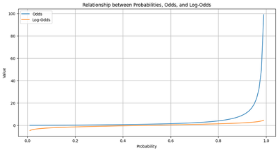
The following Python code visualizes the relationship between probabilities, odds, and log-odds using a line graph. Here’s a detailed explanation of each section of the code:
-
Import necessary libraries: The code starts by importing two essential libraries:
numpyfor numerical operations andmatplotlib.pyplotfor creating a graph. -
Define functions for computing odds and log-odds: Two functions are defined:
compute_odds(p): This function takes probabilitypas input and returns the corresponding odds value calculated using the formulap / (1 - p).compute_log_odds(odds): This function takes odds as input and returns the log-odds value using the formulanp.log(odds).
-
Create a range of probabilities: Using
np.linspace(), the code creates an evenly spaced range of probability values from 0.01 to 0.99, consisting of 100 data points. -
Compute odds and log-odds: The code uses the previously defined functions to compute odds and log-odds values for the given range of probabilities.
-
Plot the graph: The code sets up a plot titled “Relationship between Probabilities, Odds, and Log-Odds” with the following elements:
- Two lines are plotted on the same graph: one for odds and another for log-odds as a function of probability.
- The x-axis is labeled “Probability”, representing the input probability values.
- The y-axis is labeled “Value”, representing either the odds or log-odds values corresponding to each probability point.
- A legend is displayed to differentiate between the two lines (Odds and Log-Odds).
- Gridlines are added to make it easier to read the graph.
The resulting graph visualizes the relationship between probabilities, odds, and log-odds. As the probability increases, both odds and log-odds also increase, but the rate at which they increase varies. The odds line demonstrates a nonlinear relationship with the probability, while the log-odds line exhibits a more linear trend. This visualization helps to better understand how odds and log-odds change with respect to varying probabilities.
# Import necessary libraries
import numpy as np
import matplotlib.pyplot as plt

# Define a function to compute odds from probability
def compute_odds(p):
    return p / (1 - p)

# Define a function to compute log-odds from odds
def compute_log_odds(odds):
    return np.log(odds)

# Define a range of probabilities
p = np.linspace(0.01, 0.99, 100)

# Compute odds and log-odds
odds = compute_odds(p)
log_odds = compute_log_odds(odds)

# Plot the relationship between probabilities, odds, and log-odds
plt.figure(figsize=(12, 6))
plt.plot(p, odds, label='Odds')
plt.plot(p, log_odds, label='Log-Odds')
plt.xlabel('Probability')
plt.ylabel('Value')
plt.legend()
plt.grid(True)
plt.title('Relationship between Probabilities, Odds, and Log-Odds')
plt.show()
1.3.2 Ranges of Values
For probabilities, the value ranges from 0 to 1, while odds range from 0 to infinity. These restricted ranges can pose problems for linear regression since it assumes that the target variable can take any value from negative to positive infinity. On the other hand, log-odds cater to values spanning from negative to positive infinity, making them ideal for linear regression.
1.4 Logistic Regression and Its Connection to Linear Regression
In both logistic regression and linear regression, we make predictions using a linear combination of input features. This means taking a dot product of the feature vector (𝑥) and the weight vector (𝑤), i.e., 𝑧 = 𝑥 · 𝑤 + 𝑏, where 𝑏 is the bias term. The key difference between the two models lies in their prediction targets.
1.4.1 Linear Regression
Linear regression predicts a continuous target variable (𝑦) directly:
y = x.dot(w) + b
1.4.2 Logistic Regression
Logistic regression, on the other hand, predicts the log-odds of the positive class, also known as logits (𝑧). To convert the log-odds back into probabilities, we use the logistic function (also called sigmoid function):
$$ 𝑝 = \frac{1}{1+e^{-z}} $$
For classification problems, we typically want to predict the class label (e.g., cat or dog), not the log-odds. Hence, we apply the logistic function to the logits, resulting in a probability value, 𝑝.
The logistic function can be expressed as the inverse of the logit function used to convert probabilities to log-odds, which connects logistic regression back to linear regression:
$$ logit(p) = log(\frac{p}{1-p}) $$
Now that we’ve seen how the process of logistic regression is connected to linear regression, let’s take a closer look at the logistic function, which plays a crucial role in transforming log-odds values into probabilities.
The complete process of logistic regression can be summarized as follows:
- Calculate the log-odds (logits) using a linear combination of input features: $𝑧 = 𝑥 · 𝑤 + 𝑏$.
- Convert logits to probabilities using the logistic function: $𝑝 = \frac{1}{1+e^{-z}}$.
- Make predictions based on the computed probabilities (using a threshold, typically 0.5).
The code block below demonstrates the logistic function, which is the inverse of the logit function:
- Define the
logisticfunction that takes a single argument,log_odds. This function calculates the logistic probability using the formulanp.exp(log_odds) / (1 + np.exp(log_odds)). It then returns the calculated probability value.
def logistic(log_odds):
    return np.exp(log_odds) / (1 + np.exp(log_odds))
- Create an array of sample log-odds values
[-2, -1, 0, 1, 2]using the NumPynp.arrayfunction.
log_odds_values = np.array([-2, -1, 0, 1, 2])
- Apply the
logisticfunction to the array of sample log-odds values, resulting in another array containing the corresponding probabilities.
probabilities = logistic(log_odds_values)
- Display the calculated probability values for the given log-odds values.
probabilities
Understanding and applying the logistic function is essential for implementing logistic regression in practice, as it’s used to transform log-odds values into probabilities that are more easily interpretable for classification purposes.
import numpy as np

def logistic(log_odds):
    """The logistic function, which is the inverse of the logit function.

    This function takes the log-odds and returns a probability.
    """
    return np.exp(log_odds) / (1 + np.exp(log_odds))

# Test the logistic function with some values
log_odds_values = np.array([-2, -1, 0, 1, 2])
probabilities = logistic(log_odds_values)
probabilities
array([0.11920292, 0.26894142, 0.5 , 0.73105858, 0.88079708])
In conclusion, logistic regression and linear regression share the concept of predicting an outcome using input features. However, logistic regression focuses on estimating probabilities for classification problems by using log-odds and the logistic function, while linear regression directly predicts a continuous target variable.
1.4.3 Decision Boundary in Logistic Regression
The decision boundary serves as the set of points where the predicted probability is 0.5, which corresponds to a log-odds of 0. If the log-odds are greater than 0, the positive class is predicted, and if the log-odds are less than 0, the negative class is predicted. This decision boundary appears as a hyperplane in the feature space, with its orientation and position determined by the weights learned by the logistic regression model.
Let’s consider the equation for the decision boundary:
$$ 𝑧 = 𝑥 · 𝑤 + 𝑏 = 0 $$
As the logistic function returns 0.5 when 𝑧 is 0:
$$ 𝑝 = \frac{1}{1+e^{-0}} = 0.5 $$
So, the decision boundary can be visualized as an $(n-1)$-dimensional hyperplane within an $n$-dimensional feature space, defined by the equation $𝑧 = 0$. The logistic regression model then classifies new examples based on which side of this hyperplane they fall.
Let’s create a simple example using a toy dataset to illustrate the decision boundary in a 2D feature space. We will use numpy, matplotlib, and scikit-learn libraries for this visualization.
import numpy as np
import matplotlib.pyplot as plt
from sklearn.datasets import make_classification
from sklearn.linear_model import LogisticRegression

# Create a toy dataset
X, y = make_classification(n_samples=100, n_features=2, n_redundant=0, random_state=42)

# Fit logistic regression model
lr = LogisticRegression()
lr.fit(X, y)

# Generate grid of points for plotting
xx, yy = np.meshgrid(np.linspace(-4, 4, 500), np.linspace(-4, 4, 500))
Z = lr.predict_proba(np.c_[xx.ravel(), yy.ravel()])[:, 1]
Z = Z.reshape(xx.shape)

# Plot data points and decision boundary
plt.scatter(X[:, 0], X[:, 1], c=y, cmap=plt.cm.RdBu)
plt.contour(xx, yy, Z, levels=[0.5], linestyles='--')
plt.xlabel('Feature 1')
plt.ylabel('Feature 2')
plt.title('Logistic Regression Decision Boundary')
plt.show()
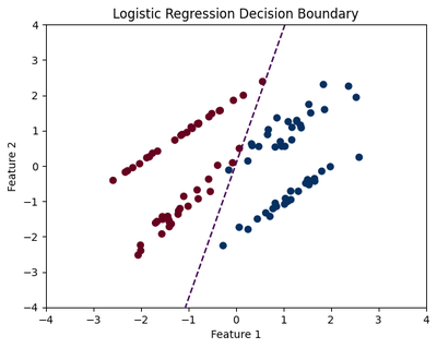
This code creates a synthetic dataset with two features and displays the fitted logistic regression model’s decision boundary. The dashed line represents the decision boundary where 𝑝 = 0.5.
Conclusion
Logistic regression and linear regression both aim to make predictions utilizing input features. However, logistic regression estimates probabilities for classification problems using log-odds and the logistic function, whereas linear regression predicts a continuous target variable directly.
Throughout this exploration, we’ve:
- Delved into the relationship between logistic regression and linear regression
- Analyzed the role of the logistic function in converting log-odds into probabilities
- Investigated the concept of a decision boundary for distinguishing classes in classification problems
- Explored how fair wages and expected winnings in gambling relate to logistic regression
- Visualized the decision boundary in a 2D feature space using Python
In future content, we will explore practical implementations of logistic regression. This will demonstrate its effectiveness in tackling real-world classification challenges. Stay tuned!